Roberto Toro, Anderson Winkler, Jason Stein
Last update: 29.Jun.2010
- Visual quality control of FSL results
- Visual quality control of FreeSurfer results
- Summary statistics, box plots and histograms
- Where to find help
1. Visual quality control of FSL results
We assume that data are organized as follows:
- Data analyses are stored in the directory
/enigma/hippo/ - The structural data was stored under
/enigma/hippo/data, with subjects namedsubj1.nii,subj2.nii, etc. - Scripts are stored at
/enigma/hippo/scripts
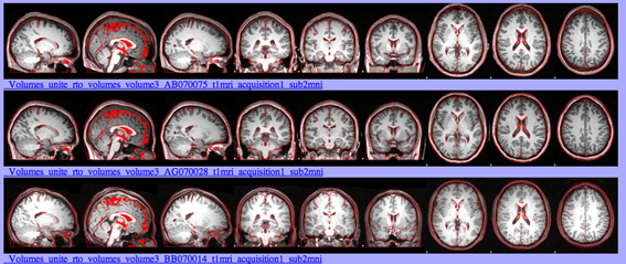
This command will produce an html page with 3 snapshots in the coronal, sagittal and axial planes of the linearly transformed volumes. For comparison, an outline of the template is drawn in red.
slicesdir -p ${FSLDIR}/data/standard/MNI152_T1_1mm.nii.gz $(imglob /enigma/hippo/*_to_std_sub.nii.gz)
- Confirm that the size of the subject brain corresponds with that of the template
- Verify that the different lobes are appropriately situated
- Confirm that the orientation of the subject matches the template
These are examples of successful linear transformations:
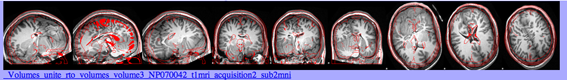
This is an example of an incorrect linear transformation:
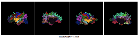
2. Visual quality control of FreeSurfer results
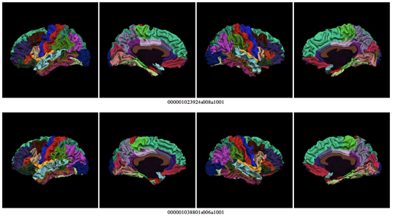
The script fsqc.sh will create a webpage with lateral and medial snapshots of white matter surface reconstructions colored with cortical labels. Clicking on the images will display a larger version. To run the script, first source FreeSurfer's environment variable $SUBJECTS_DIR to point to your subjects directory. For example:
export SUBJECTS_DIR=/enigma/hippo/fs
Next create a directory to contain the snapshots, here we will call it fsqcdir. Change the working directory to fsqcdir and run the script from there:
cd fsqcdir
source /enigma/hippo/scripts/fsqc.sh
- Check that all lobes are present, especially the ventral part of the temporal lobe
- Check that labels positions are not different from the general case
These are examples of successful reconstructions:
This is a dramatic example of an unsuccessful reconstruction:
3. Summary statistics, box plots and histograms
In R, read the hippocampal volume data.
LHippo<-read.csv("/enigma/hippo/stats/LHippo.csv")
RHippo<-read.csv("/enigma/hippo/stats/RHippo.csv")
Make a boxplot of the volumes:
boxplot(LHippo[2])
boxplot(RHippo[2])
Get the statistics used to draw the boxplot (in particular, this command will list the outlier volumes):
boxplot.stats(LHippo[2])
boxplot.stats(RHippo[2])
Now you must check all the outliers identified in this boxplot. If you are using FIRST, please examine the quality of the registration and the segmentation in the webpage generated by slicesdir (see above). Also, please manually check the segmentation of the hippocampus using fslview subj?.nii subj?_first12_all_fast_firstseg.nii.gz -l Blue-Lighblue. If you are using Freesurfer, please manually check the hippocampal segmentations using tkmedit ${subj_id} brainmask.mgz -aseg. If you decide that the segmentation is not sufficient, please remove this subject from the analysis. Please note how many subjects were removed and for what reason when uploading the results.
When you are satisfied with that the hippocampus is accurately segmented in all remaining subjects, please provide some histograms and summary statistics. First, get the statistics from the boxplot and record them. These statistics should be done after any subjects removed due to quality checking. Copy and record the outputs from these commands:
boxplot.stats(LHippo[2])
boxplot.stats(RHippo[2])
To make a histogram of the volumes and save the plots as EPS for later upload to the ENIGMA website, use:
hL = hist(LHippo[,2],xlim = c(1800,6000),nclass=100, main="Left Hippocampus",xlab="Hippocampal Volume (mm^3)")
dev.print(device=postscript, "/enigma/hippo/stats/LHippoHist.eps")
hR = hist(RHippo[,2],xlim = c(1800,6000),nclass=100, main="Right Hippocampus",xlab="Hippocampal Volume (mm^3)")
dev.print(device=postscript, "/enigma/hippo/stats/RHippoHist.eps")
The values of the histogram are also very interesting and should be recorded for later upload. These can be found by typing:
hL
hR
Next, we want to get a histogram of the left/right ratio and save the plot as an EPS for later upload to the ENIGMA website:
hist(LHippo[,2]/RHippo[,2],xlim = c(0.6,1.8),nclass=100, main="Left/Right Hippocampus",xlab="Left/Right Ratio")
dev.print(device=postscript, "/enigma/hippo/stats/LRratioHippoHist.eps")
We also want the average and standard deviation of the average bilateral hippocampal volume.
AvgBilatHippoVol = colMeans(rbind(LHippo[,2],RHippo[,2]))
mean(AvgBilatHippoVol)
sd(AvgBilatHippoVol)
Please record these values and use them for later upload to the ENIGMA website.
The same procedure should be repeated for eTIV:
hist(ICV[,2],xlim = c(600,2200),nclass=100, main="Intracranial Volume",xlab="ICV (cubic centimeters)")
If you calculated the eTIV using the 1/det method, described in these protocols - multiply your volumes by 1948.104 prior to making this eTIV histogram.
The same procedure should be repeated for brain size as well:
hist(BrainVol[,2],xlim = c(800,1800),nclass=100, main="Brain Volume",xlab="Brain Vol (cubic centimeters)")
Where to find help
General information about the ENIGMA and this protocol can be found in the consortium website:
Questions about image processing related to this project can be directed to our mailing list.
Subscribe to be informed and receive the latest updates by clicking the Join button at the top of this page.
And send emails to: enigma@lists.ini.usc.edu
General documentation and support for FreeSurfer and FSL can be found in their respective websites and mailing lists:
ENIGMA on social media: